Last time, I went step by step through training a neural network classifier in R. In this article, I’ll briefly look at three more classifiers:
- Rpart decision trees,
- Support vector machines, and
- k-nearest neighbour classification.
The bearings dataset
The diagnostic task is to classify the health of four bearings, using feature vectors derived from vibration data. There are seven health labels, with uneven numbers of samples of each class:
| early | failure.b2 | failure.inner | failure.roller | normal | stage2 | suspect |
|---|---|---|---|---|---|---|
| 966 | 37 | 37 | 608 | 4344 | 317 | 2315 |
This has a couple of implications. First, to get a true reflection of how accurate a classifier is, I need to calculate weighted accuracy, based on percentage accuracy for each class rather than total count of correct classifications. Secondly, the training set needs to be composed of equal percentages drawn from each class, and not just a randomly selected 70% of the full dataset (since this would result in very few examples of failure.b2 making it into the training set).
The neural network article discussed these points in more detail with code samples. Here, I’ll reuse the weighted accuracy function and the training set, so all classifiers here can be compared directly with the ANN and with each other.
Technique 1: Rpart Decision Trees
A decision tree is like a flow chart of questions about the features, with answers leading to more specific questions, and finally to a classification. The process of building the tree is called rule induction, with rules being derived directly from the training set of data.
Rules in decision trees are generally binary, so each will partition the data into two sets. A good rule will partition the data to minimise entropy, i.e. to maximise the certainty about which class the data belongs to. The next rule in the tree will apply only to the subset of data on that branch, which partitions the data further, and so on until enough questions have been asked to be certain about the classification.
Rpart is a decision tree implementation in R, and the code to train an rpart tree is available here. It’s simple to use, since it has very few parameters. As with the ANN, I used different penalty weights for misclassifications, to help deal with the uneven numbers of datapoints in each class. I tested three weightings:
cw1: all classes equally weighted;cw2: classes weighted by order using powers of 10;cw3: classes weighted by 1/count of samples in the dataset.
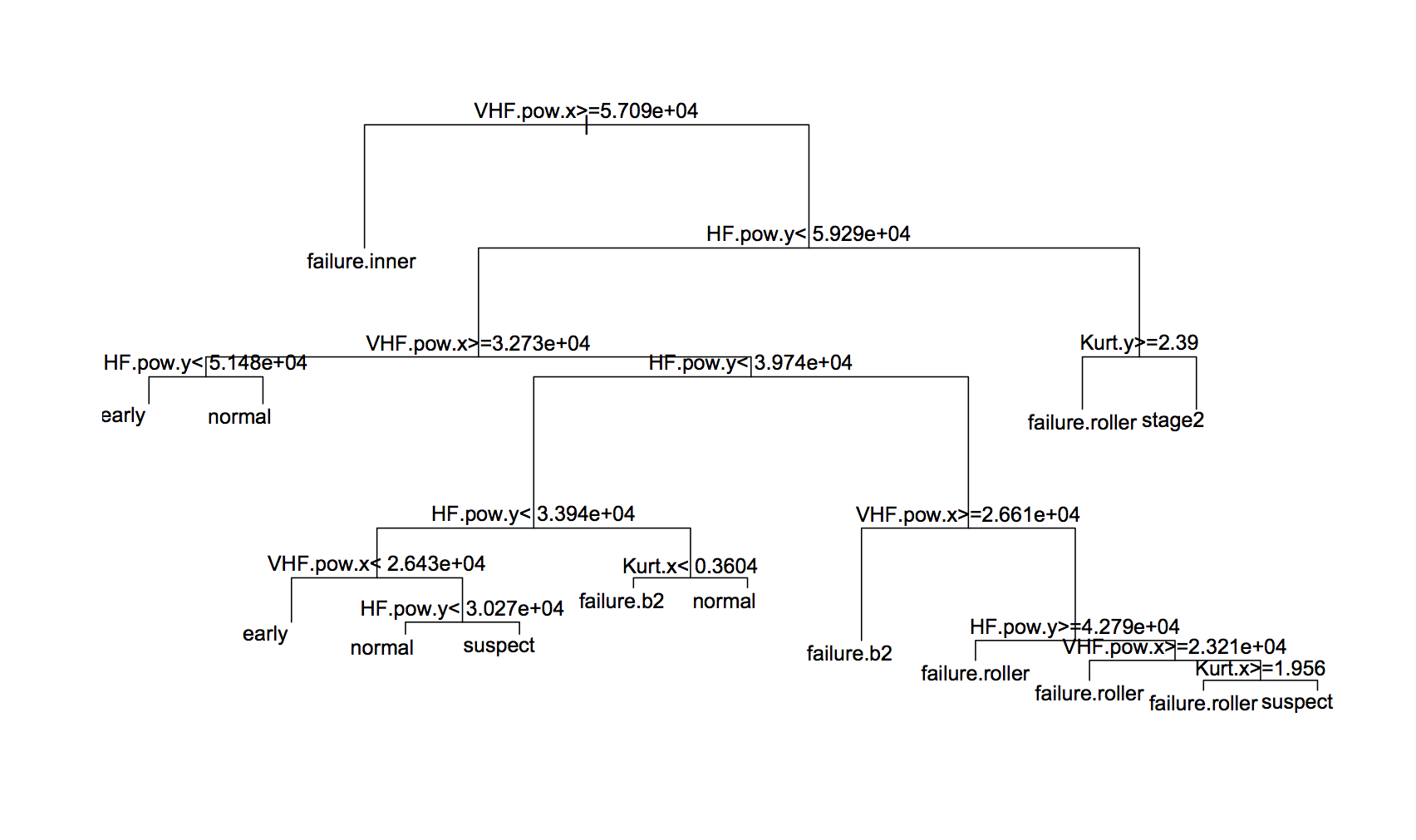
The best tree gave 90.3% accuracy, which was with cw2 weightings (although there wasn’t much difference between them). The tree itself is:
And the confusion matrix is:
| early | failure.b2 | failure.inner | failure.roller | normal | stage2 | suspect | |
|---|---|---|---|---|---|---|---|
| early | 285 | 0 | 0 | 0 | 5 | 0 | 0 |
| failure.b2 | 0 | 11 | 0 | 0 | 0 | 1 | 0 |
| failure.inner | 0 | 0 | 12 | 0 | 0 | 0 | 0 |
| failure.roller | 0 | 3 | 0 | 161 | 2 | 4 | 13 |
| normal | 186 | 0 | 0 | 0 | 1084 | 0 | 34 |
| stage2 | 0 | 0 | 0 | 1 | 1 | 94 | 0 |
| suspect | 14 | 2 | 0 | 90 | 66 | 17 | 506 |
Technique 2: Support Vector Machines
Classification is hard because it’s difficult to draw a clear boundary line between two classes. There is always some overlap between clusters of points belonging to separate classes, and it’s generally the points around the boundary that are misclassified. One way of thinking about feature design is to find parameters which maximise the distance between classes, and which minimise the number of boundary points.
Support Vector Machines (SVMs) tackle this problem by increasing the dimensionality of the data. The reasoning is that if there’s overlap between clusters in feature space, it should be easier to draw a line to separate the classes in a space of higher dimensionality. The dimensionality is increased using a kernel function, which is very often chosen to be a Radial Basis Function (RBF).
In R, SVMs can be trained using the library e1071, and my code for training is here. There are two parameters for an SVM using the RBF kernel: the cost of misclassifications, and the parameter to the RBF. A simple strategy for finding the best values for these parameters is called grid search, where you set a range on each and train an SVM for every combination of values. By comparing accuracies, you can find good combinations, and set up a second grid search using finer grained steps.
I ended up using three levels of grid search, the resulting test accuracies for which are shown below.
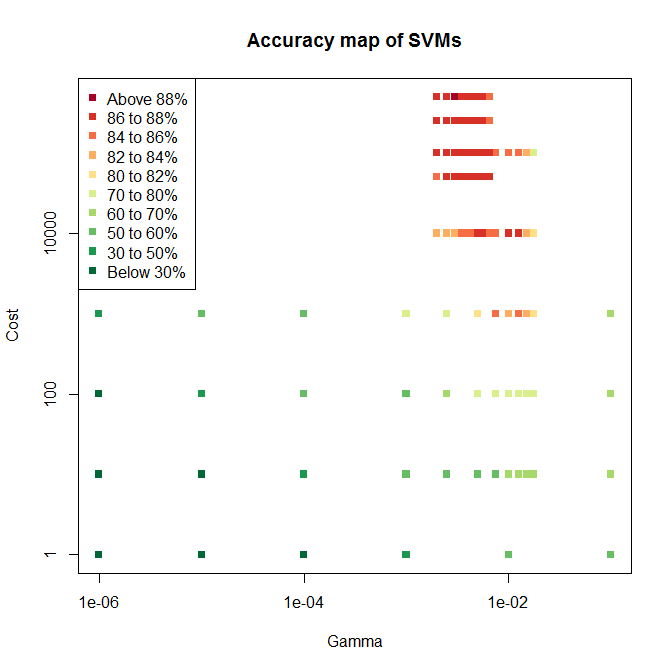
The first sweep covered six values of and four for , with mostly poor accuracy. The second sweep tried seven values of across a much tigher range, and five values for . This included two values not previously tried, since the highest accuracy on sweep one was right on the edge of the tested space. Sure enough, higher values of gave even higher accuracy, so sweep three tried higher values again, giving the cluster of mostly red points towards the top of the plot.
Since the highest accuracy is still on the edge of the tested space, there is the potential for increasing accuracy further with a fourth sweep. But SVM training is relatively computationally demanding and a sweep takes many hours, so I’ll stick with the best model found so far.
As another parameter, I also tried varying the penalty weightings applied to misclassifications. I used cw1, cw2, and cw3 from before, which gave the surprising result that cw1 tended to perform best.
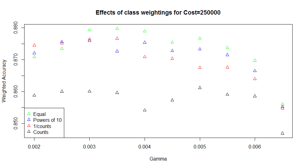
Just in case the class weightings behaved in the opposite way for the e1071 package than in other models, I also tried a cw4 set, where the counts of samples were used as weights (i.e. giving a high weight to classes with lots of samples). This gave very much poorer results (black points above), confirming that the weightings worked as expected. For the best performing SVMs, giving equal weight to misclassifications genuinely works better than proportionally penalising the minority classes.
The best SVM has an accuracy of 88.3%, with and . The confusion matrix is:
| early | failure.b2 | failure.inner | failure.roller | normal | stage2 | suspect | |
|---|---|---|---|---|---|---|---|
| early | 263 | 0 | 0 | 0 | 25 | 0 | 2 |
| failure.b2 | 0 | 10 | 0 | 0 | 0 | 0 | 2 |
| failure.inner | 0 | 0 | 12 | 0 | 0 | 0 | 0 |
| failure.roller | 1 | 0 | 0 | 133 | 3 | 9 | 37 |
| normal | 55 | 0 | 0 | 1 | 1195 | 0 | 53 |
| stage2 | 0 | 0 | 0 | 9 | 0 | 87 | 0 |
| suspect | 0 | 0 | 0 | 24 | 53 | 0 | 618 |
Technique 3: k-Nearest Neighbour
The final technique I’ll use is k-nearest neighbour, which classifies a point based on the majority class of the nearest points in feature space. The library kknn also allows weighted k-nearest neighbour, where a kernel function is applied to weight the nearest datapoints.
The two parameters for this are how many neighbouring points to take into account, ; and which kernel to weight with. The options I tried are:
- : 1, 3, 5, 10, 15, 20, 35, and 50
- kernels: rectangular (unweighted), triangular, Epanechnikov, biweight, triweight, cosine, inv, Gaussian, rank, and optimal.
Graphs of these kernels give an idea of how neighbouring points are weighted. The code for testing weighted k-nearest neighbour is here.
Since there is no iterative training of this technique, there is no way to incorporate penalty weightings for misclassifications. This has an interesting effect on the accuracy: as increases, absolute accuracy tends to increase, while weighted accuracy stays static or even decreases.
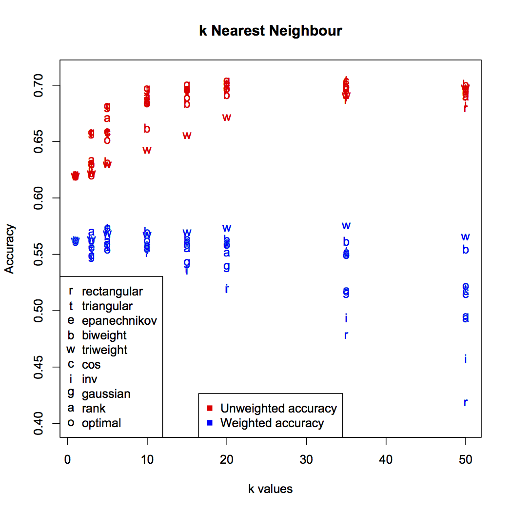
Weighted accuracy is the true reflection of the classifier’s performance. It’s an unfortunate by-product of how the technique works that the large numbers of points labelled normal and suspect will tend to dominate the nearest neighbour groups. You can see this most clearly in the weighted accuracy of the rectangular (unweighted) kernel: higher numbers of result in more normal points filling each neighbourhood, badly impacting accuracy.
The best accuracy was found to be 57.5%, with and the triweight kernel (w in the graph). The confusion matrix is:
| early | failure.b2 | failure.inner | failure.roller | normal | stage2 | suspect | |
|---|---|---|---|---|---|---|---|
| early | 115 | 0 | 0 | 0 | 166 | 0 | 9 |
| failure.b2 | 0 | 1 | 0 | 1 | 8 | 1 | 1 |
| failure.inner | 0 | 0 | 10 | 0 | 0 | 0 | 2 |
| failure.roller | 0 | 0 | 0 | 74 | 35 | 10 | 64 |
| normal | 48 | 0 | 0 | 2 | 1104 | 0 | 150 |
| stage2 | 0 | 0 | 0 | 2 | 9 | 85 | 0 |
| suspect | 3 | 0 | 0 | 11 | 274 | 5 | 402 |
Conclusions
Now I have four classifiers which each operate in different ways. The ANN finds feature weightings which distinguish one class from another. The SVM uses RBF functions to fit the non-linear function which separates classes. The decision tree produces rules to partition the data using entropy, considering one feature at a time. K-nearest neighbour assumes clusters of points are meaningful, and only considers data within the same region.
By fairly extensively exercising the parameterisation options for these approaches, I have classifiers with accuracies 94.0% (ANN), 88.3% (SVM), 90.3% (rpart), and 57.5% (k-NN).
Since the ANN is best, it’s natural to assume that 94.0% accuracy is as good as we can get on this problem. However, it’s possible to combine groups of classifiers in such a way that their overall accuracy is higher than the best individual within the group. Even the relatively poor 57.5% classifier isn’t useless! Since it behaves differently from the others, it could complement the ensemble by correctly classifying points that the others misclassify.
The choice of technique for combining different classifiers was my thesis topic, and there is an open access paper on evidence combination for the application of power transformer defect diagnosis.