Artificial neural networks are commonly used for classification in data science. They group feature vectors into classes, allowing you to input new data and find out which label fits best. This can be used to label anything, like customer types or music genres. In engineering, classifiers are often used to diagnose the health of equipment, identifying it as normal, suspect, or faulty.
The network is a set of artificial neurons, connected like neurons in the brain. It learns associations by seeing lots of examples of each class, and learning the similarities and differences between them. This is thought to be a similar process to how the brain learns, with repeated exposure to a pattern forming a stronger and stronger association over time.
This article shows how to train a neural network in R to recognise the state of health of a bearing, using features previously extracted from an open bearing dataset.
The classification problem
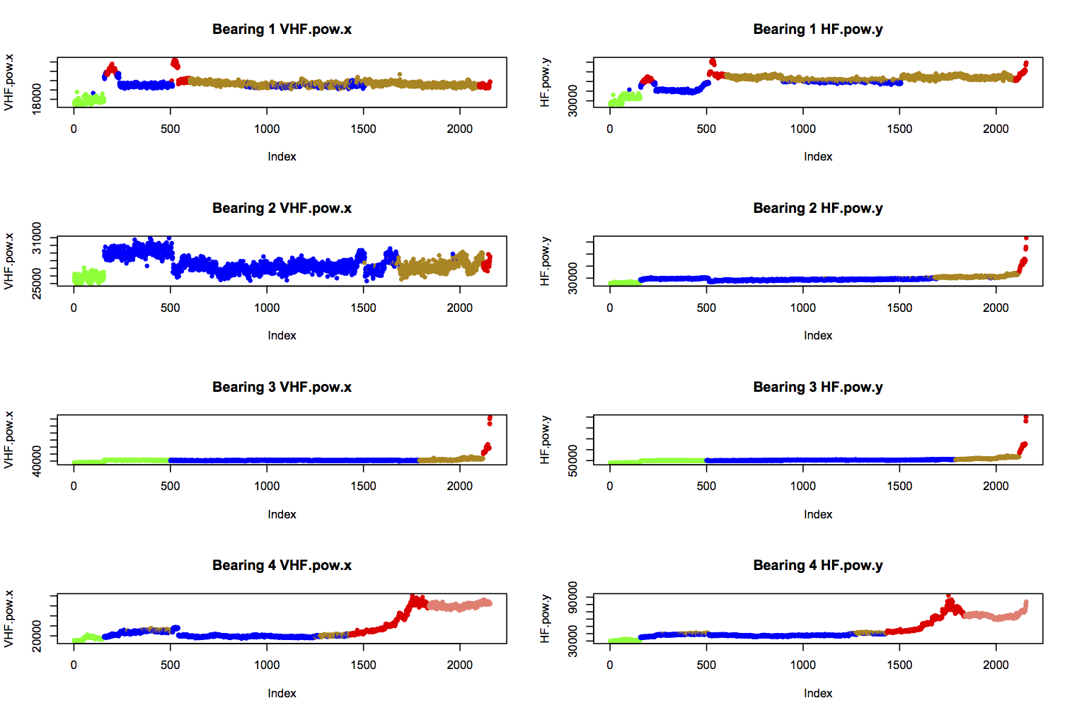
The task is to correctly diagnose the state of health of a bearing, given 14 features calculated from its vibration profile. Visual inspection and k-means clustering of data from four bearings suggested seven different states of health. These are colour-coded as follows, and shown for two features below:
- green: “early” (initial run-in of the bearings)
- blue: “normal”
- yellow: “suspect” (health seems to be deteriorating)
- red: “failure.b2”, “failure.inner” (b3), or “failure.roller” (b1 and b4)
- salmon: “stage2” (secondary failure of b4)
If you followed the last article and found your own good k-means model, you can adapt this code on GitHub to relabel the data according to the clusters you found. Then this snippet of code will read in the relabelled data for neural network training:
basedir <- "../bearing_IMS/1st_test/"
data <- read.table(file=paste0(basedir, "../all_bearings_relabelled.csv"), sep=",", header=TRUE)
Artificial Neural Networks (ANNs)
An ANN can learn patterns in data by mimicking the structure and learning process of neurons in the brain. They are widely used for all sorts of engineering problems, since it’s been shown they can approximate any non-linear function without the designer having to know beforehand what the function looks like. This is very handy, since it’s rare that an engineering problem will turn out to be linear, quadratic, or some other simple shape.
Designing a network is something of an art, since there are lots of parameters which can be tweaked, and no general design methodology for picking the best options. Often, trial and error is required to see which options give the most accurate network for a given problem.
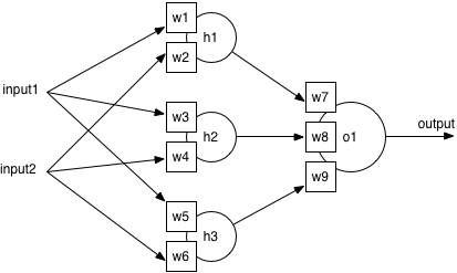
The standard ANN architecture has three layers: an input layer where features are fed in, an output layer with one neuron per class, and a hidden layer of neurons. The bearings dataset has 14 features and 7 different class labels, so automatically I know the neural network will have 14 inputs and 7 outputs. I’ll have to try different numbers of hidden neurons to be sure of the best architecture.
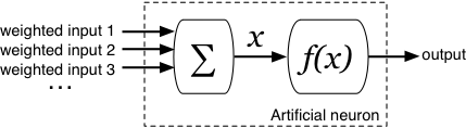
All neurons are identical in structure, and contain a sum unit and a function unit. The next section shows the maths of how a neuron turns inputs into an output value: it’s not complex, but you can go straight to how training works if you prefer.
What does a neuron do?
The inputs to the neuron are summed to give a single value, . This is then input to the function, and the output of the neuron is the output of the function, .
There are a number of functions which can be used in neurons, including the Radial Basis Function or a simple linear function, but the most common is the sigmoid or logistic function, calculated by:
This function looks like this:
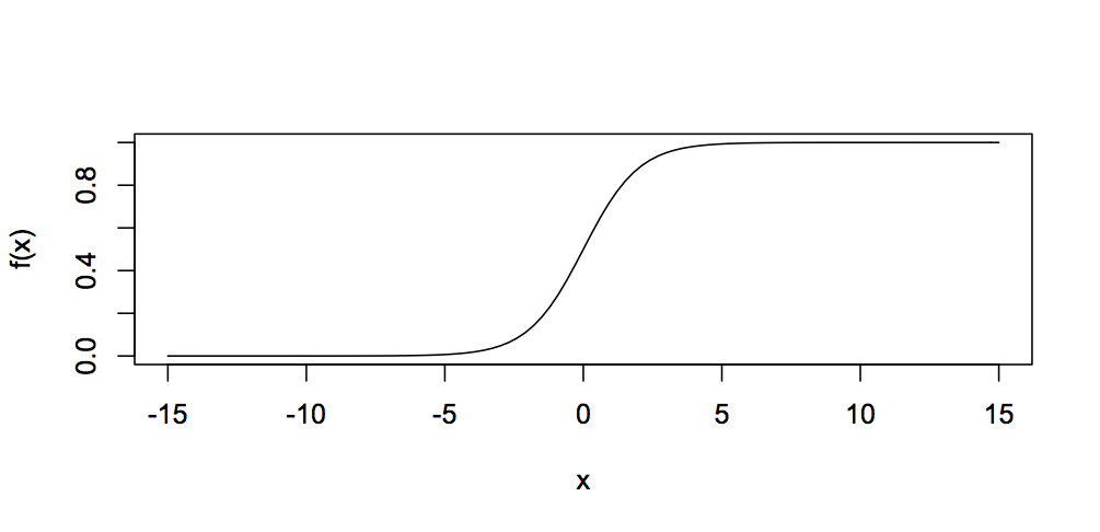
You can see that it always gives a value between 0 and 1, so the output of a neuron can only ever be in the range 0 to 1.
From this information, the result of each output neuron can be calculated. For the example network, the output of neuron is:
And , , and can each in turn be calculated:
This example network has a single output neuron, so it is making a binary classification (e.g. is the bearing faulty or not). For the actual network with seven output neurons, each is allocated to a class (early, normal, suspect, etc.). Since each output neuron contains a sigmoid function, the final output of the network is seven numbers between 0 and 1. The highest number is the winner, and the final diagnosis is the class associated with that neuron.
Training the network
So if all the neurons are identical, how does the network differentiate between classes? The answer is in the weights assigned to neuron inputs. A feature can have a large or small weight, varying the contribution it makes to the sum in any neuron. In fact, a feature can have a large weight feeding into one neuron and an almost zero weight feeding into another, meaning it has a strong influence on the first and practically none on the second.
The sigmoid function means that the neuron’s output switches from zero to one when its value crosses a threshold. This can happen in various ways, such as if one highly weighted input has a high value, or if a collection of medium weighted inputs have high values. Training the network is the process of finding the best values of weights to maximise the accuracy of classification.
The algorithm used for training is called backpropagation, and a graphical look at how it works is available here. At a high level, samples of data are shown to the network, and the error between the network’s guess classification and the actual class is used to update all the weights that led to that error. For example, if the network is shown data from a bearing classified as “early” and it diagnoses “normal”, the weights along the “normal” path will be nudged down a little and the weights along the “early” path will be nudged up a little. This makes it more likely the diagnosis will be correct the next time it sees that pattern.
A training iteration, or epoch, is when the network has been shown every sample of training data one time. Training continues over multiple iterations, until the weights reach a steady state value, or a maximum number of iterations is reached.
One possible pitfall is for the network to overtrain or overfit, which means it learns the training data set with a very high accuracy, but performs very poorly on data it hasn’t seen before. When this happens, the network has essentially memorised the training set, but can’t generalise to new data. To overcome this problem, it’s standard to split the whole dataset into a training set and a test set. After training with the training set, the network’s accuracy on the test set is calculated. The test accuracy is taken as the measure of network accuracy.
Using nnet in R
The package I’ll use is nnet, which lets you construct standard ANNs with one hidden layer of sigmoid function neurons. Even with those choices fixed, there are still a lot of parameters to tweak. This section explores those choices.
First, I construct the formula for classification. In this case we want to classify bearing State using all features as inputs. The data still has the bearing label in column 1 (b1, b2, b3, or b4), which shouldn’t be used for classification. Therefore, the basic call is:
nnet(State ~ ., data=data[,-1])There are two parameters which have always given me better results when changed from their defaults. One is to add a small decay to the weights, so they decrease over time unless reinforced by new data. The second is to increase the maximum number of iterations before training halts, from 100 to 200. These tweaks may be beneficial because the number of features I’m using makes for a larger network than may be expected, so it can take a little longer than usual to settle to a good state. This gives a call of:
nnet(State ~ ., data=data[,-1], decay=5e-4, maxit=200)The next parameter is the number of hidden neurons to use, h. There are some rules of thumb people use, such as never more than twice the number of inputs or 1/30 of your training samples, but these are not specific enough to reliably give a good result. Given the type of problem I’m trying to solve, I’m going to try every number between 2 and 30.
One final point to remember is that the starting weights are randomly assigned when training begins. Sometimes you can get particularly good or bad starting points, where the weights begin near global or local minima. I always train with the same set of parameters three times, to be more certain of getting an average-to-good starting point.
These parameter options apply to just about any ANN problem. But there are two aspects of the bearings data that complicate the task of training an ANN, and so the parameters have to be chosen more carefully. These are considered below.
Feature Vector scale
The features in the feature vector have vastly different scales from each other, and different ranges. At one end, x-axis skew values fall between -2.54 and 2.16; while at the other extreme, VHF power falls between 16,677 and 166,444. Looking at the sigmoid function, you can see that it really only changes value within a very narrow range of inputs, around -5 to +5. Using the raw data to train, the ANN has to cover a very wide possibility space of weights to find appropriate values, making tiny changes to match skew, while making massive changes to adapt to VHF power.
There is a parameter to nnet called rang, which helps to cope with this. The guidance in the help file says that initial weights are set within with rang defaulting to 0.5, but if you have large inputs, you should set rang so that:
The trouble is that this will suit the large features like VHF power well, but a modified scale will not suit smaller ones like skew very well. However, it can be applied like this:
ann <- nnet(State ~ ., data=data[,-1], size=h, rang=(1/max(data[,-c(1,2)])), decay=5e-4, maxit=200)Another approach is to normalise the dataset, so all data is scaled to fall within the range -1 to +1. This makes all features comparable in range and scale, and the nnet defaults should be more applicable. The code looks like this:
normed <- cbind(data[,1:2], as.data.frame(lapply(data[,-c(1,2)], function(col) { col / max(abs(col)) })))
ann <- nnet(State ~ ., data=normed[,-1], size=h, decay=5e-4, maxit=200)
The only way to be sure of which approach works best is to train some networks and inspect the results. I tested networks with h between 2 and 30, and did three test runs each for using normalised data, changing the rang parameter, and doing neither. The accuracy looks like this:
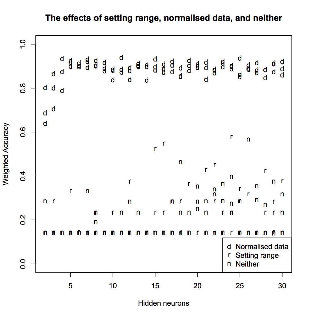
You can see that normalising the data gives significantly better results than setting the range. In some cases, setting the range gives better results that doing neither, but not consistently enough that it can be considered a good solution. For all further analysis, I’ll use only the normalised data.
Uneven counts of each class
In an ideal classification problem, there would be equal numbers of training samples from each of the classes we’re trying to learn. In almost all engineer problems, you have far more normal and healthy data than you have examples of faults and failure. The bearings dataset is a classic example of this.
For the labels I’ve assigned, the counts in each class are:
| early | failure.b2 | failure.inner | failure.roller | normal | stage2 | suspect |
|---|---|---|---|---|---|---|
| 966 | 37 | 37 | 608 | 4344 | 317 | 2315 |
If all seven classes were equally likely to occur, we’d expect a classifier making a random selection to be accurate 1 in 7 times, or 14.3%. But using this dataset, if a bad classifier were to always label everything as normal, it would be accurate 4344/8624 = 50.4% of the time! It’s like a weather prediction which always says there will be no snow tomorrow: it may be right 99% of the time, but it’s completely useless in practice.
With such uneven counts in each class, training will tend to pull the classifier towards always diagnosing the dominant class. There are two things we can do to counter this: even out the numbers in each class, or change the training to weight errors differently depending on the class label.
The first is sometimes the easiest path to take, since you can cut your dataset down to samples from each class, where is the number of samples in the minority class. However, in this case is 37, which is very small compared to the full dataset. I’d be concerned that a random selection of 37 points wouldn’t give the full range of behaviours contained in some of these classes.
The alternative is to weight errors in the ANN by different amounts. During training, when the ANN makes an incorrect classification, the size of the error affects how much the network weights are updated. I can scale this based on the class of the error, so that a missed diagnosis of failure.inner causes the weights to be updated by more than a missed diagnosis of normal.
This approach has further implications for setting up a training set, and calculating accuracy. Taking a random sample of 70% of the full dataset may result in a training set with no examples of the minority classes. I want to make sure I have 70% of the data from each class, so I wrote some R code to generate a balanced training set. I also need to write a weighted accuracy function, which calculates a percentage accuracy per class (instead of an overall accuracy dominated by “normal” classifications). The weighted accuracy function looks like this:
weighted.acc <- function(predictions, actual)
{
  freqs <- as.data.frame(table(actual))
  tmp <- t(mapply(function (p, a) { c(a, p==a) }, predictions, actual, USE.NAMES=FALSE)) # map over both together
  tab <- as.data.frame(table(tmp[,1], tmp[,2])[,2]) # gives rows of [F,T] counts, where each row is a state
  acc.pc <- tab[,1]/freqs[,2]
  return(sum(acc.pc)/length(acc.pc))
}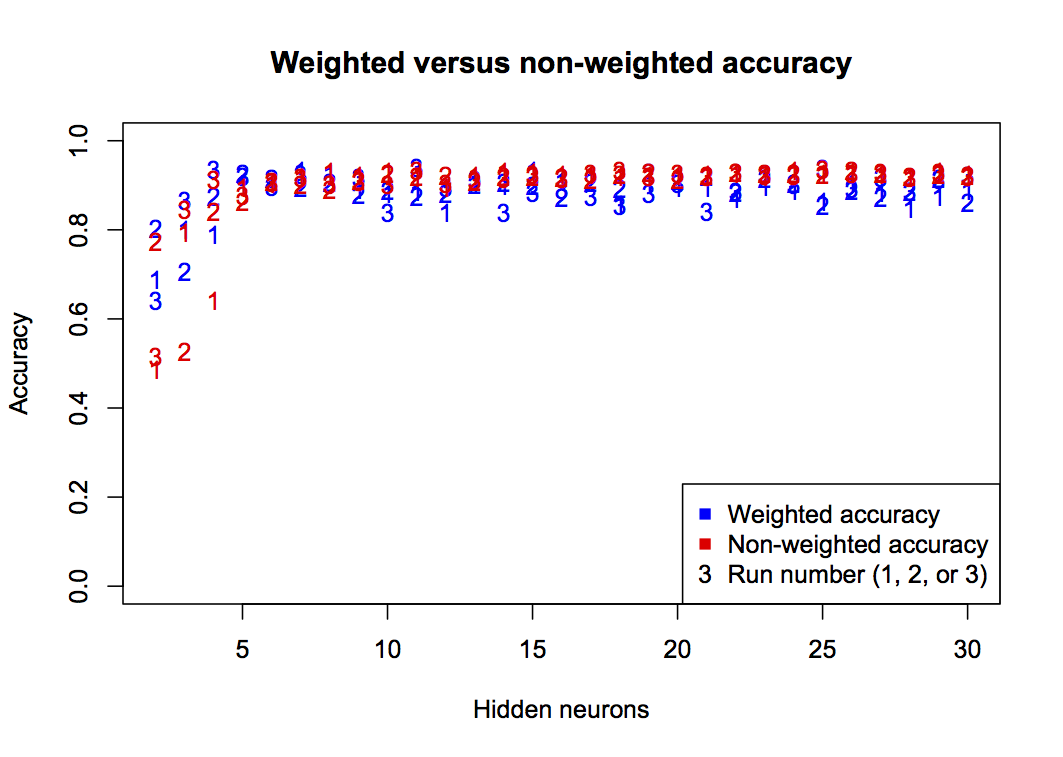
This graph shows that non-weighted (standard) accuracy gives a consistently high value, especially at h>5. But this is not a true representation of accuracy considering the unequal class counts, so the blue points give a more practical interpretation of classifier accuracy. For future graphs, only the weighted accuracy will be shown.
Now I have a training set and accuracy function, I can train networks using class error weightings. I’ll try three different options: all classes equally weighted, classes weighted by order using powers of 10, and classes weighted by 1/count of samples in the dataset:
cw1 <- rep(1, 7) # all equal
cw2 <- c(10, 100, 100, 10, 1, 10, 1) # powers of 10
freqs <- as.data.frame(table(data$State))
cw3 <- cbind(freqs[1], apply(freqs, 1, function(s) { length(data[,1])/as.integer(s[2])})) # 1/counts

class.weights <- rbind(cw1, cw2, cw3[,2])
colnames(class.weights) <- c("early", "failure.b2", "failure.inner", "failure.roller", "normal", "stage2", "suspect")

for (i in 1:3)
{
  for (c in 1:length(class.weights[,1]))
  {
    data.weights <- do.call(rbind, Map(function(s)
      {
        class.weights[c,s]
      }, data$State))

    for (h in 2:30)
    {
      ann <- nnet(State ~ ., data=data[train,-1], weights=data.weights[train], size=h, decay=5e-4, maxit=200)

      pred <- predict(ann, data[,-1], type="class")
      tacc <- weighted.acc(pred[train], data[train,2]) # weighted training accuracy
      wacc <- weighted.acc(pred[-train], data[-train,2]) # weighted test accuracy

      results <- rbind(results, c(h, tacc, wacc, c))
      models[[(length(models)+1)]] <- ann
    }
  }
}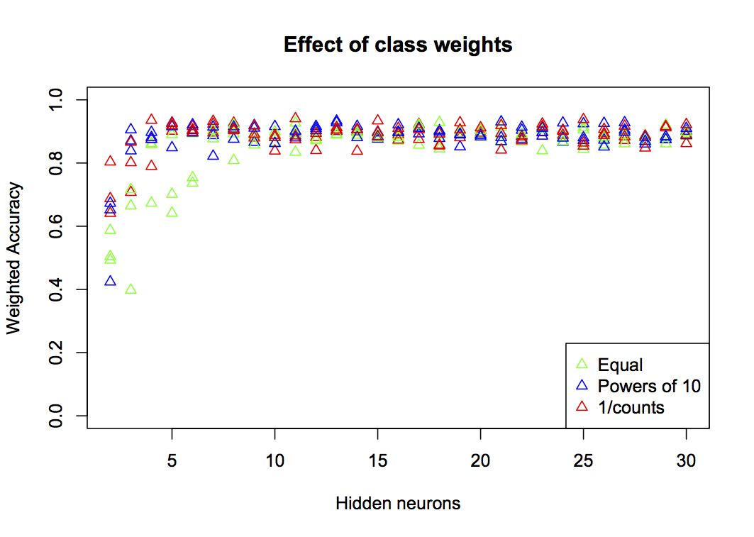
You can see that at low numbers of neurons (h<10), equal weighting performs very much worse than the other two. There’s not much to choose between the simplified powers of 10 and the programmatically derived 1/counts, so either will work well as a solution.
Results
The full code to test all the options above can be downloaded here. After running, I found the best network was generated by:
- Normalising the data
- Taking account of the uneven class counts, by:
- Selecting a balanced training set
- Calculating weighted accuracy
- Applying class weightings to errors
- Using class weightings of 1/counts
- Using 11 hidden neurons.
This network gives a weighted accuracy of 94.0%, and the confusion matrix below:
| early | failure.b2 | failure.inner | failure.roller | normal | stage2 | suspect | |
|---|---|---|---|---|---|---|---|
| early | 280 | 0 | 0 | 0 | 10 | 0 | 0 |
| failure.b2 | 0 | 11 | 0 | 0 | 0 | 1 | 0 |
| failure.inner | 0 | 0 | 12 | 0 | 0 | 0 | 0 |
| failure.roller | 0 | 0 | 0 | 163 | 0 | 2 | 18 |
| normal | 71 | 0 | 0 | 1 | 1213 | 0 | 19 |
| stage2 | 0 | 0 | 0 | 0 | 0 | 96 | 0 |
| suspect | 0 | 0 | 0 | 34 | 11 | 0 | 650 |
This shows a dominant diagonal of labels assigned correctly to samples. Generally speaking, there are small levels of confusion between early and normal data, with 10 early points being classed as normal, and 71 normal points classed as early. There is also some confusion between suspect and failure.roller samples.
It is encouraging that there is very little confusion between the classes relating to good health and those of bad health. One single normal point is misclassified as a fault class, and none of the early points. In addition, the failure classes are only ever misclassified as other types and stages of failure, never as normal behaviour. There is most confusion about the suspect class, but this is understandable if we consider suspect to be a transition between good and bad health.
Conclusion
I’ve quite comprehensively experimented with various parameters for training a neural network to recognise the state of health of the bearings. The accuracy is good at 94.0%, but not perfect.
One approach to increasing this accuracy is to train other types of classifier, to see if anything performs significantly better than the ANN. There are lots and lots of different techniques so this is always worth investigating.
A rougher engineering approach is to classify a number of sequential datapoints, and take a majority view of the likely state. For example, if three sequential feature vectors are classified as normal, it’s highly likely the bearing is in a normal state. If two are classified as failure.inner and one as suspect, we can be more sure of the fault diagnosis than if we just look at one classification in isolation. Particularly for an engineering system which changes fairly gradually over time, this can be a simple but effective method of increasing certainty in the result.