There’s growing interest in opening up civic datasets, to let local communities do interesting and new analyses. This article shows how to map Toronto sidewalks by neighbourhood, using City of Toronto open data, Google Maps, and R.
Background
I took part in the Open Toronto Open Data Book Club last week. This is a neat idea where an open dataset is chosen at the start of the month, and data scientists bring along their analyses to the meetup for a show-and-tell. Discussion takes place around what was good about the dataset, what could be improved, and what further analysis could take place.
The dataset for last week’s meeting was the City of Toronto Sidewalk Inventory, which lists the type of sidewalk present on all streets in Toronto. It codes street segments based on whether there is sidewalk on both sides, one side only, or no sidewalk, and also includes information on pathways, laneways, and other walkable spaces.
I presented colour coded maps of sidewalks by city neighbourhood, giving a visualisation of how good the sidewalk coverage is in each part of town. This article breaks down the R code to do this.
Getting the neighbourhood data
First step was to load in the Toronto neighbourhoods dataset, which is another open dataset curated by the City of Toronto. The neighbourhoods are provided as a Shapefile, which can be read in R using the readShapeSpatial function from the maptools library.
areas <- readShapeSpatial("neighbourhoods2", CRS("+proj=longlat +datum=WGS84"))When I first downloaded the neighbourhoods Shapefile and tried to load it, I got the following error:
> readShapeSpatial("NEIGHBORHOODS_WGS84"))
Error in getinfo.shape(fn) : Error opening SHP file
To solve this, I opened the Shapefile up in QGIS and re-saved it (without doing anything else), and this fixed the problem for me (nice 😎).
Getting the sidewalk data
Next, I had to load in the sidewalk data. This is also provided as a Shapefile, so I used readShapeSpatial again. However, the data is currently tagged with the wrong projection information, so I added a custom projection string:
projection <- "+proj=tmerc +lat_0=0 +lon_0=-79.5 +k=0.9999 +x_0=304800 +y_0=0 +ellps=clrk66 +units=m +no_defs"
sidewalks <- readShapeSpatial("Sidewalk_Inventory_wgs84", proj4string=CRS(projection))
The second issue I ran into is that the sidewalk position co-ordinates are given in eastings and northings, whereas the neighbourhood positions are in latitude and longitude. Thankfully, there is an spTransform function in the library rgdal that can convert between the two!
sw.lat.long <- spTransform(sidewalks, CRS("+proj=longlat +datum=WGS84"))Now I have my neighbourhoods and sidewalks on the same co-ordinate system, I can start doing some analysis!
Finding sidewalks inside a given neighbourhood
The Toronto neighbourhoods have a unique 3-digit code, as well as unique names. One of the core downtown neighbourhoods is the Bay Street Corridor, with code 076. You can get all the data associated with this one area as follows:
nh <- areas[areas@data$AREA_S_CD=="076", ]
cat(paste0("Area is ", nh$AREA_NAME, "\n"))
nh.pts <- fortify(nh)
What does that last line do? Well, the neighbourhood nh is an object of type SpatialPolygonsDataFrame: a complex data structure that includes co-ordinate and projection information, the area name and code, and a representation of the polygon defining the neighbourhood boundary. The fortify function essentially flattens this object into a tabular format, where each row represents a single point in the polygon. The table has columns for latitude and longitude of the point, amongst other features. This tabular format is needed for plotting on the map later, so I’ll return to it shortly.
In the meantime, the next step is to find which of the sidewalks exist inside the chosen neighbourhood. The over function can do this for us!
inside <- !is.na(over(sw.lat.long, as(nh, "SpatialPolygons")))
sub <- subset(sw.lat.long, inside)
As long as you downgrade the neighbourhood object to a SpatialPolygons first, over returns one entry per sidewalk, either 1 (inside) or NA (outside the neighbourhood polygon). If you just pass in nh as is, you end up with a table of results with one row per sidewalk, but columns for each of the attributes in nh. The values are still either 1 or NA, just repeated across the columns.
I convert this to a list of true and false values with !is.na, then use that list to subset out only those sidewalks that are inside the neighbourhood. We’re getting close!
Colour coding the sidewalks
The original sidewalk dataset codes each entry by the type of sidewalk in place:
- Sidewalk on south side only
- Sidewalk on north side only
- No sidewalk on either side
- Sidewalk on west side only
- Sidewalk on east side only
- Pending (Roadway under construction)
- Sidewalk on both sides
- Not used
- Not used
- Laneway without sidewalks
- Walkway (pedestrian path documented in the City road data)
- Pathway (pedestrian path not documented by the City)
- Not applicable (a feature where no sidewalk is expected, e.g. expressway)
There are 13 different codes, and I don’t want my maps to have such fine-grained detail. I’m just interested in whether the road segment has sidewalks on both sides, one side, or none, and I want to colour code those as green, amber, and red. So I mapped these sidewalk codes into my own scheme as follows:
sdwlk <- c("ok", "ok", "bad", "ok", "ok", "other", "good", NA, NA, "other", "good", "good", "other")I decided to include a fourth category called other, for the situations where red/amber/green isn’t really applicable. I’ll colour these blue so they can be seen without distorting the impression of sidewalk coverage.
Next comes the most complex bit of code. I mentioned before that the fortify function is used to convert a complex SpatialPolygonsDataFrame object into a more-straightforward tabular format of points which can be drawn on a map. This includes latitude and longitude, but loses the sidewalk code attribute SDWLK_Code. I need to assign a known unique id to each of the sidewalks, so that I can merge the sidewalk code information back in to the fortified points. I then derive a sidewalk coverage indicator for each point based on the sidewalk code and my coverage scheme sdwlk:
sub@data$id <- rownames(sub@data)
sub.pts <- fortify(sub)
sub.pts <- merge(sub.pts, sub@data, by="id")
coverage <- sdwlk[sub.pts$SDWLK_Code]
sub.pts <- cbind(sub.pts, coverage)
At this stage, I have all the information needed to map the sidewalks!
Mapping the result
The library ggmap lets you easily download Google Maps for areas at various zoom levels using qmap. The following code downloads a map, then plots the neighbourhood boundary and colour-coded sidewalks on top of it:
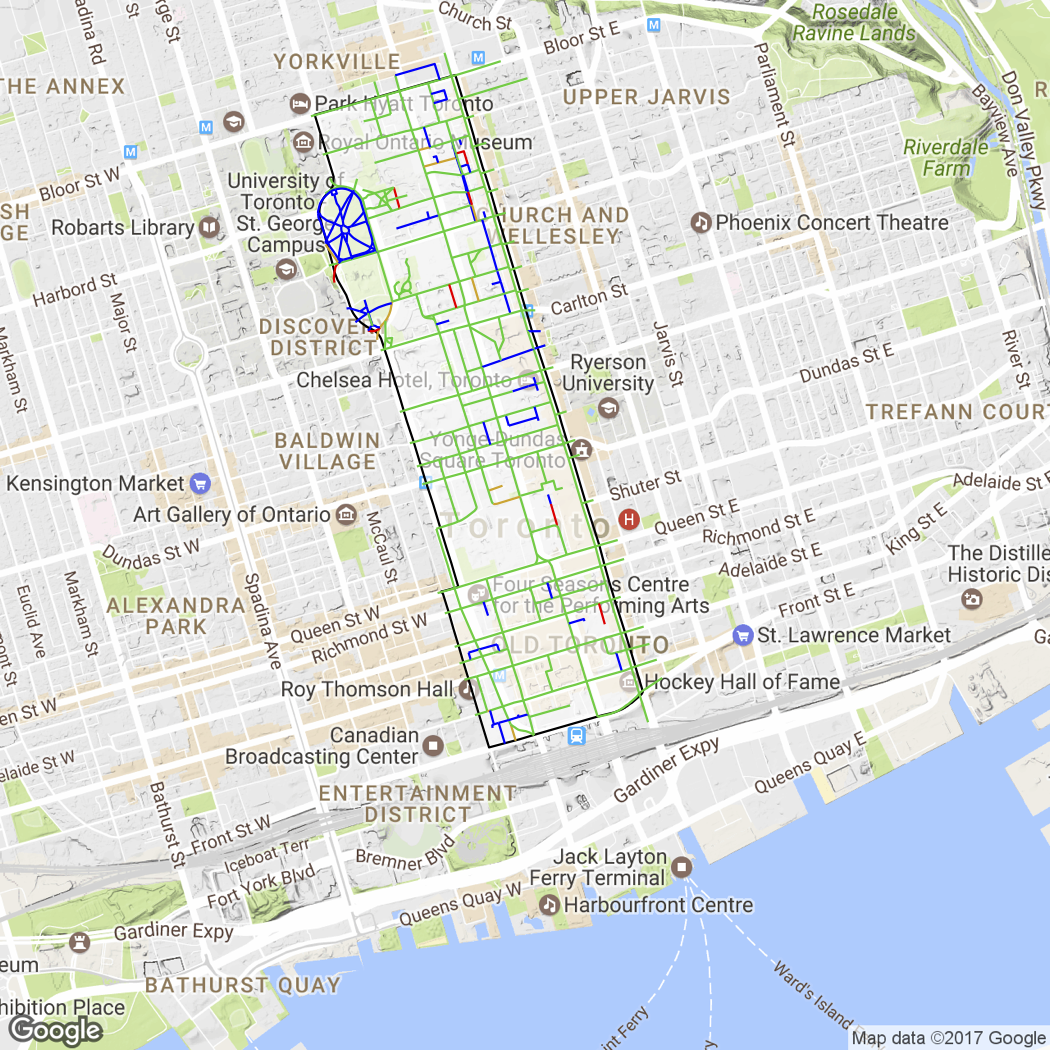
toronto <- qmap("Toronto, Ontario", zoom=14)
toronto +geom_polygon(aes(x=long, y=lat, group=group, alpha=0.25), data=nh.pts, fill='white', show.legend=F) \
  +geom_polygon(aes(x=long, y=lat, group=group), data=nh.pts, color='black', fill=NA, show.legend=F) \
  +geom_path(aes(x=long, y=lat, group=group, color=coverage), data=sub.pts, show.legend=F) \
  +scale_colour_manual(values=c("good"="#00CC33", "ok"="goldenrod", "bad"="red", "other"="blue"))
You can see that this uses the fortified versions of both the neighbourhood and the sidewalks for plotting. By passing the color=coverage parameter to geom_path, I’m saying that I want the colour of each sidewalk to be dependent on its coverage code. However, I also need the scale_colour_manual part at the end of this line to assign specific colours to each code, otherwise a default colour scheme is used.
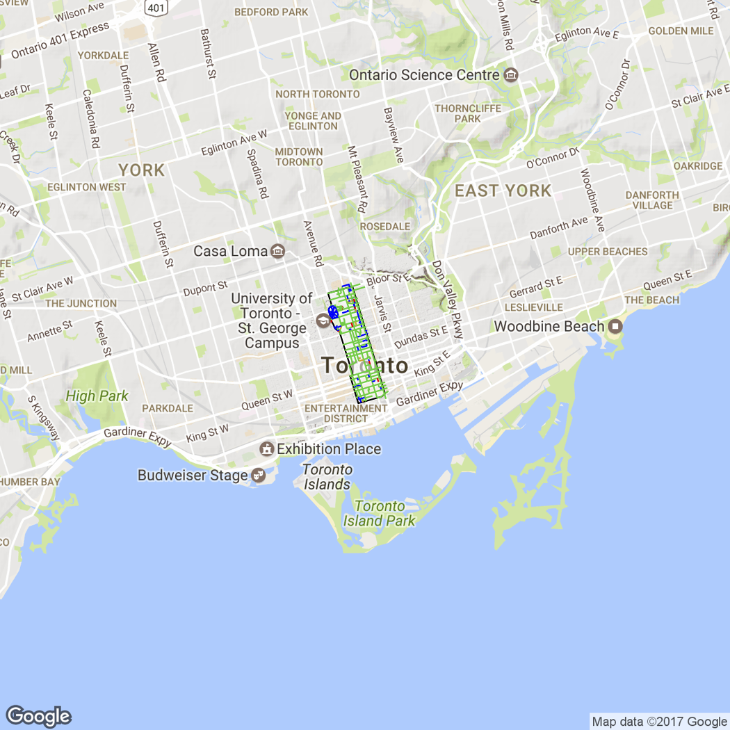
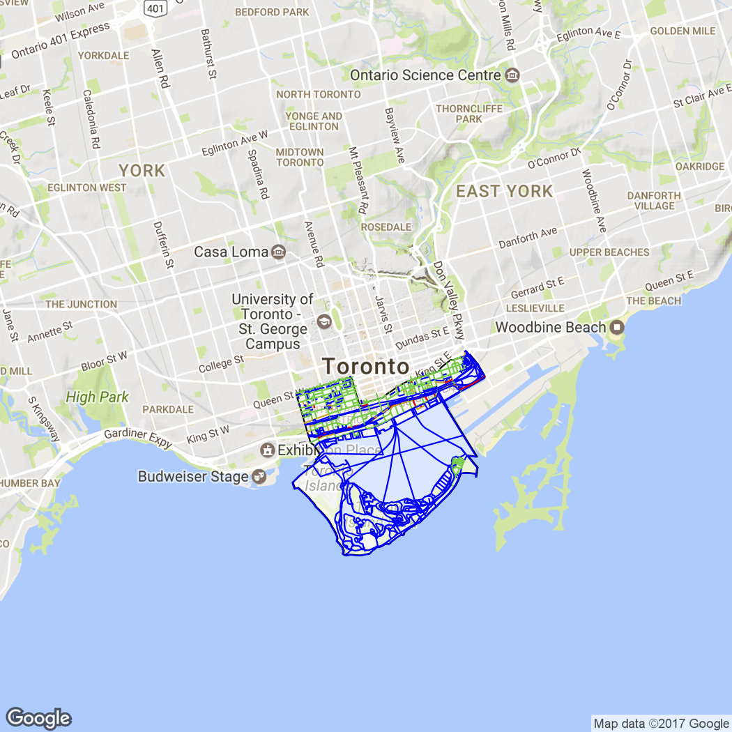
Output
Now it’s time to explore different neighbourhoods! The Bay Street Corridor is right in the heart of downtown Toronto, and as may be expected, the sidewalk coverage is very good. The Waterfront Communities are also a core area, and have similarly good coverage. However, once you get a bit further out from downtown, the coverage can drop off quite badly. The Maple Leaf neighbourhood, for example, shows a lot of red and amber.
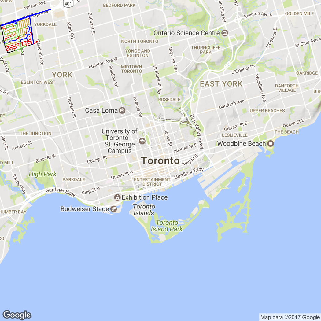
The full code is available on GitHub, so you can go ahead and explore your own neighbourhood!