Linear regression in Rust

Rust is an interesting new programming language, with a rich type system, zero-cost abstractions, and a memory-safety checker. The best way to pick up a new programming language is to build something real with it. Also, the best way to understand how a machine learning algorithm really works is to build it yourself.

I decided to learn both Rust and the inner workings of linear regression at the same time. Linear regression is a simple concept, but still very useful for data science. This article describes the algorithm and its applications, and what I learned while building it in Rust.

What is linear regression?

A common use of linear regression is to fit sampled data to a straight-line function of the form:

$y = mx + c$

where $x$ is the input value and $y$ is the corresponding output value, $m$ is the slope of the straight line and $c$ is the constant or y-intercept value.

As a machine learning task, you would generally start with a dataset of $(x, y)$ pairs and an idea that they have a linear relationship. The challenge is then to find the values of $m$ and $c$ which best fit the data, which is where linear regression comes in. Once you have these parameters, you can use the straight line model to generate values of $y$ for any new $x$ .

As an example, let’s assume that we’ve collected the following data:

$$x$$	0	1	2	3	4	5
$$y$$	0.1	1.9	6.2	11.9	21.0	30.1

Performing linear regression on this gives an $m$ of 6 and a $c$ of -3.33, which looks like this:

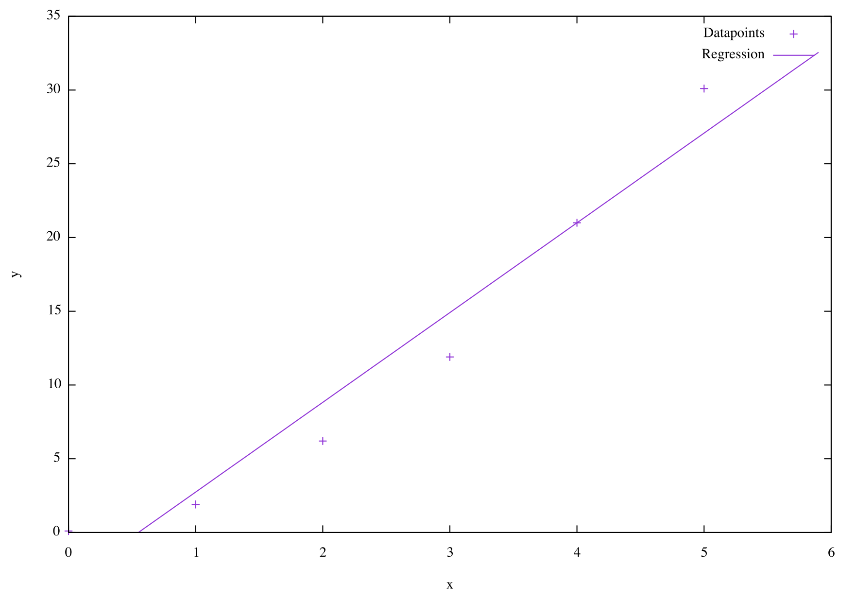
You can see that the data doesn’t fit perfectly to a straight line. There is either some error on our data, or it’s not a perfect straight line relationship between our $x$ and $y$ values.

Fitting a straight line is one use of linear regression, but it’s also more powerful than that. It can fit any model where the output $y$ is dependent on one or more inputs $x_i$ . So we can fit any of the following models:

$\begin{eqnarray} y & = & m_1x_1 + m_0 \\ y & = & m_2x_2 + m_1x_1 + m_0 \\ y & = & m_3x_3 + m_2x_2 + m_1x_1 + m_0 \end{eqnarray}$

We can even use linear regression to fit polynomial models:

$\begin{eqnarray}y & = & m_2x^2 + m_1x + m_0 \\ y & = & m_3x^3 + m_2x^2 + m_1x + m_0 \end{eqnarray}$

Hold up, how can linear regression fit a non-linear polynomial? Well, the technique considers the three input variables separately; that is, the dependent variable $y$ is linear with respect to each of $x^2$ , $x^1$ , and $x^0$ . Each $m_i$ parameter scales its input linearly. The model only cares about finding the $m_i$ parameters, and doesn’t know or care that the input variables have a non-linear relationship to each other.

So what does a higher-order polynomial fit on our example data look like? If we perform the regression to a second order polynomial (a quadratic) we get the parameters $m_0 = 0$ , $m_1 = 1$ , $m_2 = 1$ , which looks like this:

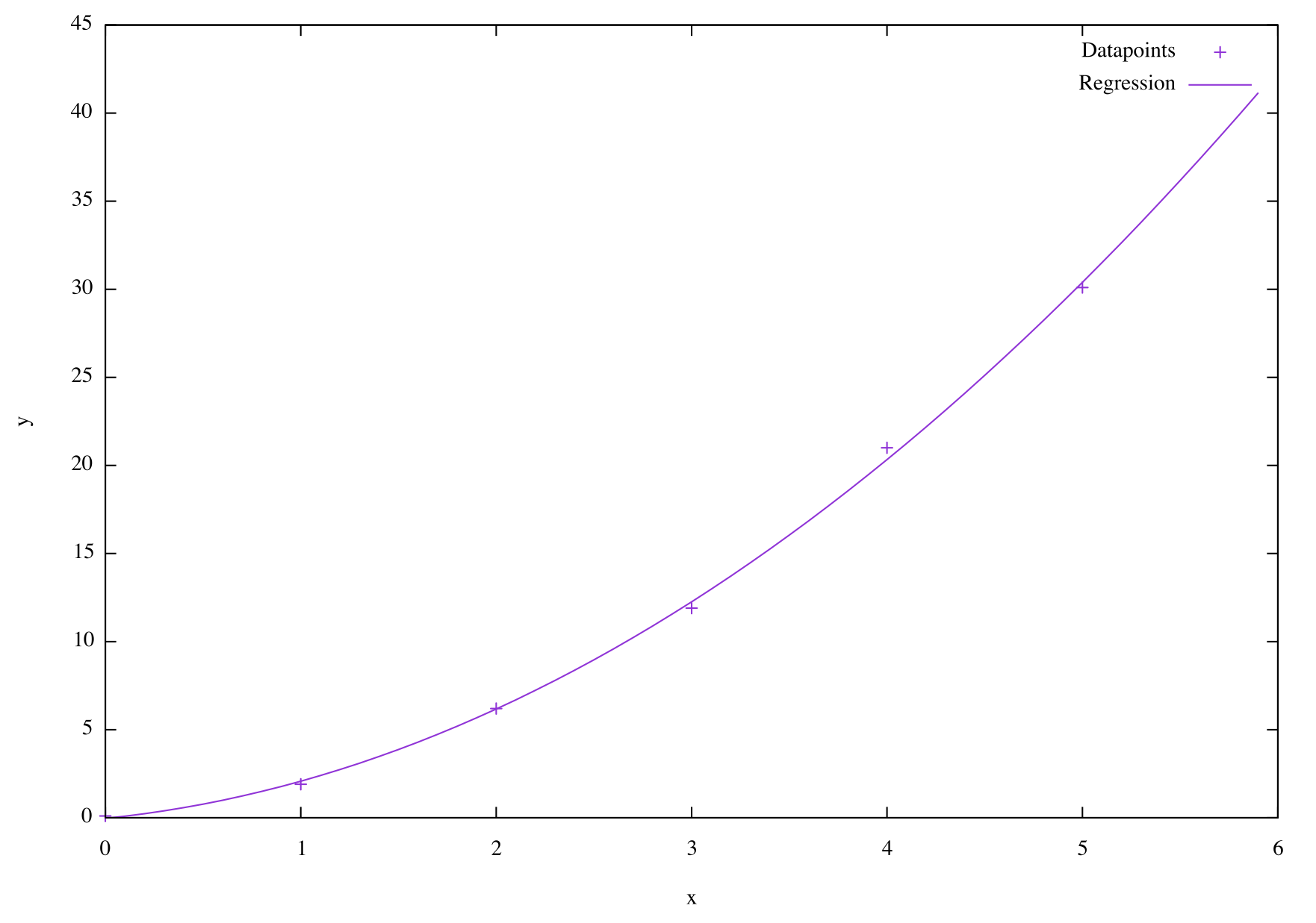
Much better!

Matrix representation

The general problem we are trying to solve with linear regression can be written as:

$\mathbf{y} = \mathbf{x \beta} + \mathbf{e}$

where $\mathbf{y}$ is a vector containing $n$ datapoints, $\mathbf{x}$ is a matrix of $n$ datapoints with $d$ dimensions, $\mathbf{\beta}$ is a vector of $d$ parameters, and $\mathbf{e}$ is a vector of $n$ error values.

For the first order polynomial case (a straight line), the equation for the $i$ th datapoint simplifies to:

$y_i = \left[ \begin{array}{cc} 1 & x_i \end{array} \right] \left[ \begin{array}{c} \beta_{0} \\ \beta_{1} \\ \end{array} \right] + e_i$

And for the quadratic it would be:

$y_i = \left[ \begin{array}{ccc} 1 & x_i & x_i^2 \end{array} \right] \left[ \begin{array}{c} \beta_{0} \\ \beta_{1} \\ \beta_{2} \\ \end{array} \right] + e_i$

Linear regression aims to find the vector $\mathbf{\beta}$ for a given set of $\mathbf{y}$ and $\mathbf{x}$ values. Note that if we are fitting a polynomial, our dataset will give us the complete $\mathbf{y}$ vector, but only a single dimension of the $\mathbf{x}$ matrix (the $\mathbf{x^1}$ dimension). We can automatically populate the remaining $d-1$ dimensions of the $\mathbf{x}$ matrix by squaring, cubing, etc each $x_i^1$ value as required, and setting the first column to all 1s.

There are a few different ways of estimating the $\mathbf{\beta}$ matrix. One of the most stable is called Singular Value Decomposition (SVD), and it’s the one we’ll use here.

SVD allows us to decompose the $\mathbf{x}$ matrix into three matrices:

$\mathbf{x} = U S V$

As before, the $\mathbf{x}$ matrix has dimensions $n \times d$ . If $\mathbf{x}$ has rank $r$ , then the $U$ and $V$ matrices are $n \times r$ and $r \times d$ respectively, and have the following properties:

$U^T U = I$ $V^T V = I$

The dimensions of $S$ and $I$ are both $r \times r$ , and $S$ is a diagonal matrix. Often, the rank of $\mathbf{x}$ will be equal to the order of the polynomial, meaning $r = d$ .

Once we have calculated the three matrices $U$ , $S$ , and $V$ , the final step is to use them to estimate the values of $\mathbf{\beta}$ . If we go back to our general equation, we can substitute in the SVD matrices as follows:

$\mathbf{y} = \mathbf{x \beta} + \mathbf{e}$ $\mathbf{y} = U S V \mathbf{\beta} + \mathbf{e}$

Let:

$\alpha = S V \mathbf{\beta}$

Then the following estimation can be defined:

$\hat{\alpha} = U^T \mathbf{y}$

Finally, we can rearrange the first equation again to get estimates of $\beta_j$ for $j$ from 1 to $d$ :

$\hat{\beta_j} = \sum\limits_{k=1}^{d} v_{jk} \frac{\hat{\alpha}_k}{s_{kk}}$

For full details of these derivations, please see “Use of the Singular Value Decomposition in Regression Analysis” by J. Mandel.

Linear regression in Rust

Ok! Now we know what we’re aiming to do, it’s time to start writing some Rust. There are three stages to the program:

Reading in the data
Performing the linear regression
Visualising the result

These are explained in detail with code snippets below. If you want to see the whole thing up front, the complete program for linear regression in Rust can be found here.

The one short-cut I’ll take is to use the la library for representing matrices and performing the SVD decomposition. This is because the Matrix type has helpful functions, and the calculations for the three SVD matrices are a bit tedious. If you are very keen, please check the source for the SVD calculations here.

Reading data in Rust

The first step is to read in some data. The file format we’ll use is a CSV, where each row represents one datapoint, and each datapoint has an x value and a y value. We want to read this data into a Matrix, with the same meaning for rows and columns.

We can start by taking the data filename as an argument to the program, parsing the file, and exiting if any problems are encoutered.

fn main() {
    let args: Vec<String> = env::args().collect();
    let filename = &args[1];
    let data = match parse_file(filename) {
        Ok(data) => data,
        Err(err) => {
            println!("Problem reading file {}: {}", filename, err.to_string());
            std::process::exit(1)
        }
    };
}

The parse_file function needs to open the file, read the CSV format (using the Rust csv library), and decode each line into two 64-bit floating point values (for the x and y co-ordinates). It then assembles those lines into a one-dimensional vector, because that’s the format the Matrix constructor needs:

fn parse_file(file: &str) -> Result<Matrix<f64>, Box<Error>> {
    let file = try!(fs::File::open(file));
    let mut reader = csv::Reader::from_reader(file).has_headers(false);

    let lines = try!(reader.decode().collect::<csv::Result<Vec<(f64, f64)>>>());
    let data = lines.iter().fold(Vec::<f64>::new(), |mut xs, line| {
        xs.push(line.0);
        xs.push(line.1);
        xs
    });

    let rows = data.len() / 2;
    let cols = 2;
    Ok(Matrix::new(rows, cols, data))
}

If the program executes up to this point, we can guarantee that we have a Matrix of (x,y) values ready for the next step.

Performing the linear regression

In order to get our data into the right format, we need to extract an $\mathbf{x}$ matrix and a $\mathbf{y}$ matrix. The $\mathbf{y}$ matrix is simple enough, as it is just a column matrix of the y values of each datapoint:

let ys = data.get_columns(data.cols()-1);

The $\mathbf{x}$ matrix is a little more complex. It needs to have the right number of columns for the order of the polynomial we are trying to fit. If we’re trying to fit a straight line (order 1), we need two columns: one to represent values of $x^1$ and one to represent $x^0$ (i.e. $x$ and 1). If we’re trying to fit a quadratic (order 2), we need three columns: one each for $x^2$ , $x^1$ , and $x^0$ .

The x values from our file are the $x^1$ values. For any order of polynomial we need to add a column of 1s to the left of the $x^1$ column. For polynomials of a higher order than 1, we also need to add corresponding columns to the right of the $x^1$ column.

For example, if we start with the x values from above and want to fit a quadratic, the $\mathbf{x}$ matrix should end up as:

$\left[ \begin{array}{ccc} 1 & 0 & 0 \\ 1 & 1 & 1 \\ 1 & 2 & 4 \\ 1 & 3 & 9 \\ 1 & 4 & 16 \\ 1 & 5 & 25 \\ \end{array} \right]$

This can be achieved with:

let xs = generate_x_matrix(&data.get_columns(0), order);

and the function:

fn generate_x_matrix(xs: &Matrix<f64>, order: usize) -> Matrix<f64> {
    let gen_row = {|x: &f64| (0..(order+1)).map(|i| x.powi(i as i32)).collect::<Vec<_>>() };
    let mdata = xs.get_data().iter().fold(vec![], |mut v, x| {v.extend(gen_row(x)); v} );
    Matrix::new(xs.rows(), order+1, mdata)
}

This looks scary at first glance, but it’s really not so bad! This function does three things:

Creates a function gen_row which takes one parameter x, and returns a vector of values of $x^i$ . i runs from 0 up to order inclusive, so this function will generate a row of the $\mathbf{x}$ matrix with the right number of columns for a given polynomial order.
For each value in xs, call the new function gen_row and concatenate together all the resulting values.
Reshape the concatenated values into a Matrix of appropriate dimensions.

The final step is to calculate the $\mathbf{\beta}$ vector, as follows:

let betas = linear_regression(&xs, &ys);

The corresponding linear_regression function does a few different things:

Use the la library to perform SVD, and extract the corresponding u, s, and v matrices,
The s matrix is returned with dimensions $n \times r$ , although all rows after row $r$ contain zeros. Cut the s matrix down to size ( $r \times r$ ) and call it s_hat,
Calculate the vector of $\hat{\alpha}$ values and call it alpha,
Divide all values in alpha by the corresponding value in the diagonal matrix s_hat, and format the vector back into a Matrix,
Multiply all these values by the corresponding value in v.

fn linear_regression(xs: &Matrix<f64>, ys: &Matrix<f64>) -> Matrix<f64> {
    let svd = SVD::new(&xs);
    let order = xs.cols()-1;

    let u = svd.get_u();
    // cut down s matrix to the expected number of rows given order
    let s_hat = svd.get_s().filter_rows(&|_, row| { row <= order });
    let v = svd.get_v();

    let alpha = u.t() * ys;
    let mut mdata = vec![];
    for i in 0..(order+1) {
        mdata.push(alpha.get(i, 0) / s_hat.get(i, i));
    }
    let sinv_alpha = Matrix::new(order+1, 1, mdata);

    v * sinv_alpha
}

That’s all there is to it! The resulting values in betas are the estimated parameters of the model.

Visualising the results

The best way to assess how well the model fits the data is to graph it. Graphing and visualisation are not native to Rust, so for this final step I will use the Rust Gnuplot library.

The examples of how to use the library are really nice and clear, so I won’t go into detail here. The only tricky bit is that you can’t plot the model as a function directly. Instead, we can generate (x, y) pairs of points along the function, and plot those as a series. I did this in four steps:

Generate a function for the line:

let line = { |x: f64| (0..(order+1)).fold(0.0, |sum, i| sum + betas.get(i, 0) * x.powi(i as i32))};

Calculate the maximum x value of the function based on the input data:

let max_x = data.get_columns(0).get_data().iter().fold(0.0f64, |pmax, x| x.max(pmax) ) + 1.0;

Create a series of x values between 0 and max_x in steps of 0.1:

let mut x_steps = vec![];
for i in 0..(max_x as usize) {
    for j in 0..10 {
        x_steps.push((i as f64) + 0.1 * (j as f64));
    }
}

Generate the corresponding y values for each x using the function line:

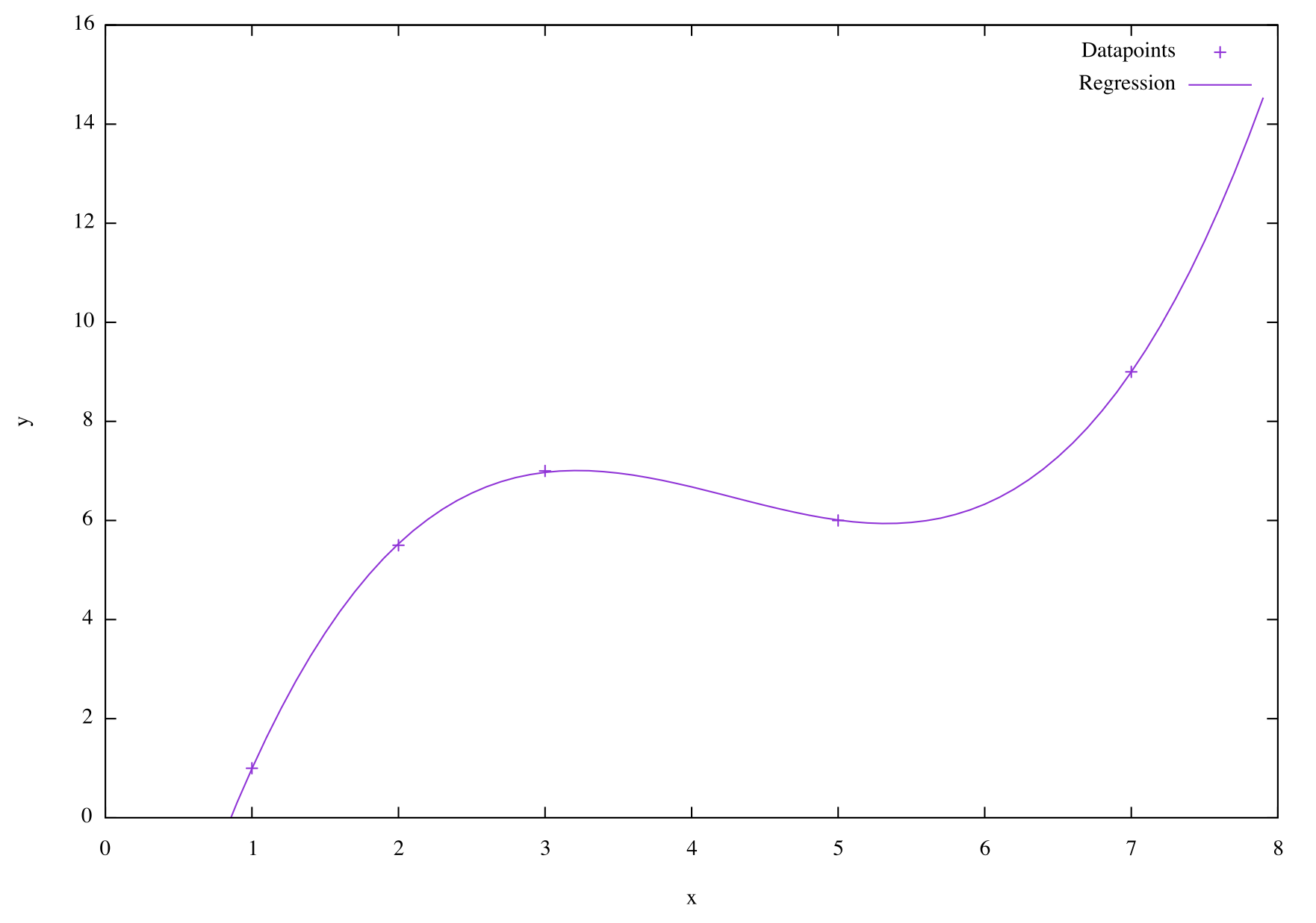
let y_steps = x_steps.iter().map(|x| line(*x) ).collect::<Vec<_>>();

The final step is to create the figure, with both datapoints and the regression line shown:

let mut fig = Figure::new();
fig.axes2d().points(data.get_columns(0).get_data(), 
                    ys.get_data(), 
                    &[Caption("Datapoints"), LineWidth(1.5)])
    .set_x_range(AutoOption::Fix(0.0), AutoOption::Auto)
    .set_y_range(AutoOption::Fix(0.0), AutoOption::Auto)
    .set_x_label("x", &[])
    .set_y_label("y", &[])
    .lines(x_steps, y_steps, &[Caption("Regression")]);
fig.show();

Which can generate something like this!

Final thoughts

The goal of this was to learn some Rust and get a deeper understanding of linear regression at the same time. I feel I’ve succeeded with both of these, and I’m always happier using a technique on a dataset if I fully understand what it is doing. The full program for linear regression in Rust can be found here.

Two of the things I really like about using Rust are the explicit typing, and explicit mutability. From the first, I know that if my program runs, every function is accepting and returning exactly the type of variable that I intended it to. From the second, I know that I’m only making changes to variables I have intentionally marked as mut. While these features don’t eliminate bugs entirely, I can be a lot more certain that I haven’t accidentally switched variable names, and I’m performing operations on the data I think I am.

In total, these features help me to be more confident that a running program is a correct program. While a test suite can build confidence that certain inputs are handled correctly, tests plus the type system and memory checking give confidence that the program will work as intended for all inputs.

Linear regression in Rust

What is linear regression?

Matrix representation

Linear regression in Rust

Reading data in Rust

Performing the linear regression

Visualising the results

Final thoughts

You might also like